Thinking, Fast and Typed

Daniel Kahneman gave us a vocabulary most of us now use without crediting him. Thinking, Fast and Slow divided the mind into two characters. System 2 is the deliberate one: it works through an argument, checks itself, holds a number in memory, and gets tired doing it. System 1 is the fast one. It knows a face before you have decided to look, hears that a room has gone quiet, and answers most of your day without being asked.
Kahneman's point was that we run on System 1 far more than we like to admit, and that most of the time it is right.
The analogy only goes so far, and psychologists have spent years arguing about how clean the two-system split really is. But it is a useful handle for something true about the machines. A large language model thinks by writing: one token at a time, each conditioned on the last. That is what makes it good at open problems, and it is the only mode it has.
Now watch an agent work for an hour. It reads a ticket and decides which team owns it. It looks at a tool call and decides whether to run it. It reads a retrieved passage and decides whether it answers the question. It reads its own draft and decides whether it is finished.
Four decisions. Four short lists. Not one of them needs a paragraph.
We answer all of them with the deliberate machine.
Not because nobody thought of the alternative. We have had discriminative models for as long as we have had machine learning, they pick a label and attach a probability, and they are very good at it. What changed is that agents made every one of these decisions trivially easy to express as a prompt and comparatively annoying to express any other way. So the generative model quietly absorbed a great deal of work it was never the best tool for.
That is the thing worth looking at directly, and something has arrived that works the other way.
What structured outputs fixed, and what they left alone
To be fair to the current state of the art: this used to be much worse. Two years ago you asked for JSON, got prose with JSON somewhere inside it, and wrote a regex. Then you handled the case where the model wrote Yes! instead of {"answer": "yes"}, and the case where it apologised first.
Constrained decoding fixed that. Every serious provider will now hand you output that validates against a schema you supply, because the decoder is prevented from emitting a token that would break it. If you are still parsing prose for decisions, you are several years behind and the fix is an afternoon.
But a schema constrains the shape of the answer, not the way it is produced. Two costs survive it.
The first is mechanical. The model is still running an autoregressive loop, generating a sequence one token at a time, each conditioned on everything before it. That is what makes a language model powerful on open problems, and it is pure overhead when the entire content of the answer is one of four labels. You pay the latency and the tokens either way.
The second is subtler and matters more. Your schema can declare a field called confidence and the decoder will faithfully guarantee that a number appears in it. Nothing in that machinery makes the number mean anything. It is a token the model emitted because the schema asked for one.
A different shape
TypeSafe released Jev into early access on 15 September, and took Kahneman's name for it: a System One model. Borrowed vocabulary is not evidence of anything, and the analogy is doing marketing work as much as descriptive work. The mechanism underneath is the part worth your attention.
TypeSafe describes Jev as producing all of its outputs in one query rather than decoding a sequence. The internals are not published, so treat the mechanism as the vendor's account rather than an established fact. What you can check from the outside is the interface, and the interface is the interesting part: you hand it a state and a set of typed questions, and typed values come back with probabilities attached, with no text anywhere in the exchange.
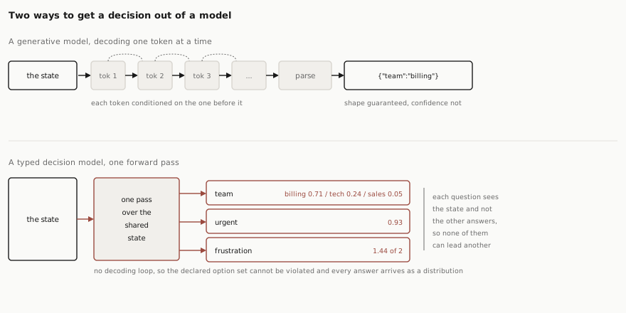
It is worth being precise about what that does and does not buy, because the obvious claim is the wrong one.
Type validity is not the differentiator. Constrained decoding already guarantees a valid answer, and a properly configured generative model will not break your schema either. Anyone selling you type safety as the reason to switch is selling you something you already have.
What differs is where the probability comes from. In the generative case, a confidence field holds a number the model wrote, chosen the way it chooses any other token. Here the number is the distribution the answer was selected from. Those are different objects that happen to print the same way, and only one of them can be calibrated in any meaningful sense.
The second difference is cost. No sequential decode means no tokens to pay for and no loop to wait on, which is what makes the economics of the next section possible.
Three primitives and one call
The interface has three question types. A yes or no. A choice from a list you define in the request. A score against a rubric you supply. Jev's choice primitive takes up to 255 options.
Here is a support ticket going through one call. The state is the ticket text. Three questions ride along: which team owns this, is it urgent, how frustrated does this customer sound.
Back comes a team with a probability across your options, something like billing at 0.71 against technical at 0.24 and sales at 0.05. Urgency comes back as a number between 0 and 1. Frustration comes back as a position on your rubric.
What happens next is yours. A valid typed answer is not a correct one, and the threshold at which you auto-route rather than escalate is a policy decision that no model makes for you. This is worth saying plainly because the typing can create a false sense that the decision has been made. It has not. The decision has been quantified.
One property here is quietly excellent. The questions share the input and are answered in isolation from each other, so the urgency answer cannot be dragged around by whatever the routing answer turned out to be. Anyone who has watched a chain-of-thought talk itself into a conclusion across three sub-questions will recognise what that buys.
It is not a classifier, and that is the whole point
Here is the objection worth taking seriously, because it is the one a good ML engineer raises immediately: we have had classifiers for decades. They output calibrated probabilities. Scikit-learn will calibrate one for you in three lines. What is new?
What is new is when the task is specified.
A trained classifier has its label set fixed at training time. The categories are baked into the weights. Changing them means gathering examples and retraining. That is entirely fine when the task is stable, and it will usually beat anything else on a fixed, well-sampled problem.
A typed decision model takes the question and the options in the request, with no examples. You can ship a new question this afternoon. That flexibility is the product, and it tells you exactly when to reach for one.
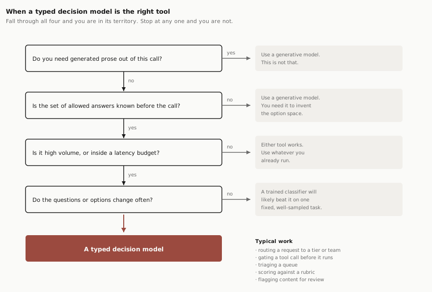
If your categories are stable and you have labelled data, train a classifier. The typed decision model earns its place when the questions move, when there is no training set, or when a new question has to exist by Friday.
The experiment that made me take the category seriously
There is a second reason this shape is interesting, and it has nothing to do with any vendor. You can see it on a laptop in a few minutes.
Take a small model you can run locally. Ask it one yes or no question about a document: does this ticket contain an instruction trying to make an agent do something it should not. Then read the answer twice, from the same call. Once as the word it wrote. Once as the probability mass sitting on Yes against No, normalised across just those two tokens, which most runtimes will return if you ask for logprobs.
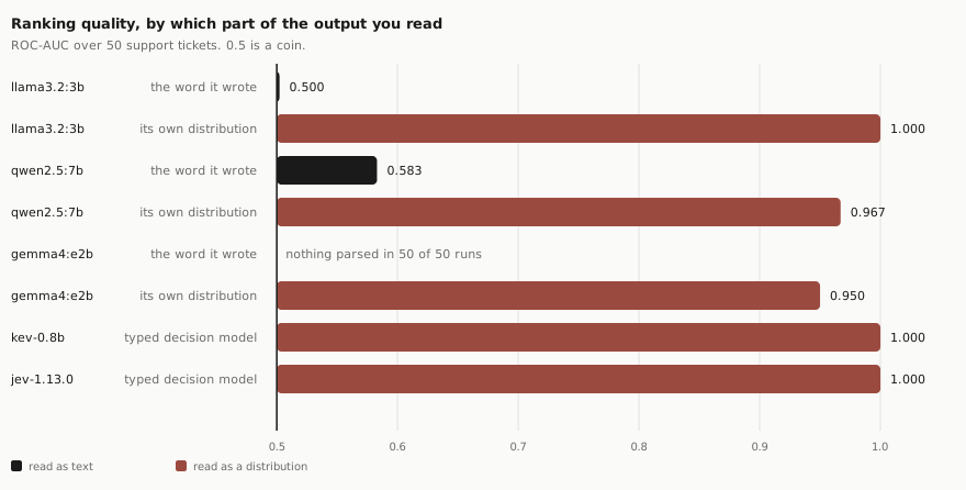
Across fifty tickets, llama3.2:3b wrote "No" fifty times. One answer, repeated, which ranks at 0.500. A coin. The distribution behind that same token ordered all fifty correctly, every injected ticket above every clean one.
Be careful what that licenses, because it is easy to over-read. It demonstrates ranking signal on this corpus. It does not demonstrate calibrated confidence, and it does not isolate the typed output head as the cause of anything, since the two typed models in that chart differ from the general models in base, training and head all at once. The corpus is fifty tickets built from six injection templates. The recovered scores averaged 0.106 on the attacks, so a 0.5 threshold still catches nothing and any threshold you had tuned against the old readout is void.
The full run is published with its limits, including the corrections it went through.
With those caveats attached, the point survives: a general model computes graded information on its way to an answer, and rendering that answer as a word throws the gradation away. Typed decision models hand you that layer directly. A good part of what the category is selling is access to something that was already being computed and discarded.
What calibration actually means
Every model in this class will advertise calibration, so it is worth being precise about the word, because it is used loosely and means something specific.
A detector is calibrated when its stated probability matches its observed hit rate. Of everything it called 0.9, about nine in ten should turn out to be right. You check it by grouping predictions by what was claimed and measuring how often each group was correct.
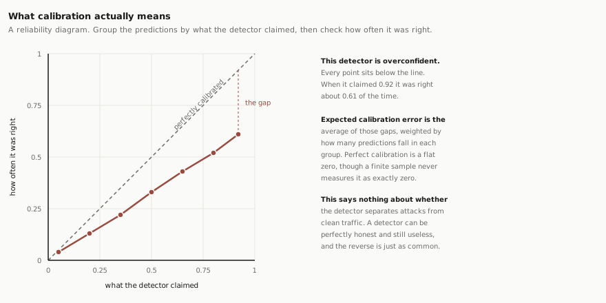
That last point deserves its own sentence, because conflating the two is the most common mistake in this area. A detector that says 0.5 about everything, on a population that is half attacks, is perfectly calibrated and completely useless. A detector that ranks every attack above every clean document can be wildly overconfident about all of them. Calibration and discrimination move independently, and a vendor citing one is not telling you about the other.
How to audit the claim
Expected calibration error, the number you will be quoted, has a property that almost nobody mentions: it is biased upward on small samples. Each group of predictions carries sampling noise, and the metric takes the absolute value of every gap, so the noise cannot cancel out.
Simulate a detector that is already perfect and it still does not measure zero.
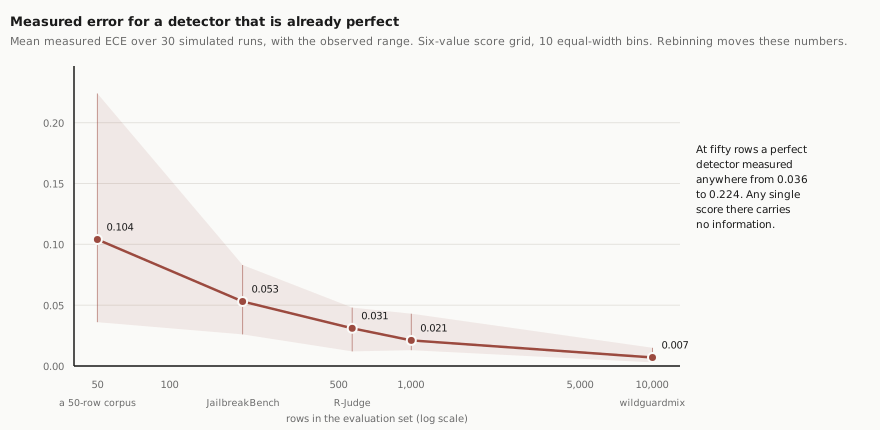
At fifty rows a perfect detector measures about 0.104 on average, and individual runs landed anywhere between 0.036 and 0.224. Now notice where the public benchmarks sit. JailbreakBench is 200 items. R-Judge is 569.
So the question to put to a vendor is not how low the calibration error was. It is how many rows it came from, and what a perfectly calibrated detector would have scored on that same evaluation under the same binning. One number without the other does not establish much.
There is a companion trap on the other side of the evaluation. Zero false positives on twenty clean documents does not mean the false positive rate is zero. The rule of three puts a rough upper bound at three in twenty, and at a realistic base rate the difference between a 0.1 percent false positive rate and a 15 percent one is the difference between a detector you can run and one that buries your reviewers. Ask how many negatives were in the evaluation, and reason about your own base rate rather than the vendor's.
What it costs you
Three things, none of them fatal, all of them worth knowing before you plan around this.
No strings. Nothing here writes. If a flow needs a summary as well as a decision, that flow needs a generative model too, and you are now running two dependencies where you ran one. That is a real architectural cost and not always worth paying.
A closed world. These models pick from options you declare. They cannot surface a category you did not think of, which is a feature when you want determinism and a wall when your taxonomy is still moving.
An unverified probability until you verify it. Everything in the section above applies to every model in the category, including the open ones, and including any number I have quoted here.
Trying it without committing to anything
Jev is live on Cloudflare Workers AI as typesafe/jev. Two things cost me an hour and are not in the documentation. Partner models are not reachable at the documented /ai/run/{model} path; they take the model in the body of /ai/run. And they do not draw on the free Workers AI allowance, so you will get an insufficient balance error until the gateway has credit. Fifty documents cost a fraction of a penny after that.
There is also an open-weight route, which I would start with. Kev is an Apache-licensed family serving the same API on localhost, and its model card publishes calibration figures next to the evaluation they came from, which is the standard worth holding everyone to. The chart above uses the 0.8B checkpoint, which is quick; the larger ones are slow on Apple silicon because the kernels have no Metal path yet.
The evaluation actually worth running is not a benchmark. Take one routing or triage decision you already make with a general model. Run both against a week of your own traffic. Compare mistakes, escalation rate, latency and cost. That answers the question for your system, which is the only place it can be answered.
The shape this points at
Everything above frames this as a choice: generative model or decision model, pick one per task. That framing is too small, and it is the part of this I expect to matter in two years when the specific vendors have shuffled.
Once both kinds of call are cheap, the question stops being which to use and becomes how they compose.
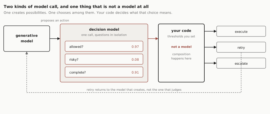
A generative model proposes. A decision model scores the proposal against several typed questions at once. Then ordinary code, holding thresholds you chose, decides what any of that means.
That third box is the one that gets skipped, and it is the one doing the governance. Nothing in the model layer knows that 0.08 risky is acceptable and 0.31 is not. That number is your risk appetite, written down, in a language you can read in a review and change without retraining anything.
TypeSafe's own interface pushes you toward exactly this. The questions are atomic, answered independently against the same state, and nothing in the API composes them for you. Their documentation is explicit that a question needing several factors weighed should be decomposed into separate questions and recombined with logic in your code. The vendor is telling you where the boundary is.
Look at the loop again and notice what the retry arrow does. It goes back to the model that creates, not the model that judges. That is the whole point of splitting them. When a proposal fails its checks, the thing that needs another attempt is the generation, and the judgement stays fixed while it happens. Ask one model to do both and a failed check becomes a conversation it can talk itself out of.
Guardrails, routing, verification, escalation and completion checks all have this shape. They have been implemented as prompts because prompts were the only available surface. None of them wanted to be prose.
What to leave with
Not that Jev is good. It is a week old, its internals are undisclosed, and its calibration claim is unverified by anyone outside the company. Not that decision models replace language models either; the first gate in that ladder sends most work straight back to a generative model, and it should.
The thing worth carrying is smaller and more durable than any of that.
An agent may need two kinds of model call: models that create possibilities, and models that choose among them. For three years we have asked one interface to do both, because it was the only interface there was. The cost of that was invisible while there was no alternative to compare it against.
Agent architectures today tend to check at one or two points. Not because one or two is the right number, but because a judgement cost real latency and real money and you could not afford one everywhere. That constraint has quietly shaped a lot of system design, including a good deal of the guardrail architecture now being sold as best practice. Move the cost far enough and more of those checks become affordable, including the ones currently skipped because the budget ran out.
Whether that changes your design is an empirical question and the answer depends on your numbers. But it is a different question from the one the field has been asking, and for the first time you can explore it on a laptop for nothing.